GPT Training Memory Estimation - NeMo Practice
1 Introduction
Training large-scale language models like GPT requires efficient memory management and optimization techniques. This article will discuss memory estimation with model hyperparameters, PyTorch memory profiling tools, and some improvements to the NeMo framework.
2 Memory Estimation with Model Hyperparameters
The memory requirements for training GPT models depend on various factors, including the number of parameters, batch size, and optimizer states. For example, a 1.5 billion parameter GPT-2 model requires 3GB of memory for its weights. The memory needed for training also depends on the optimizer used. Mixed-precision Adam, for instance, has a memory multiplier of 12, leading to a memory requirement of at least 24 GB for a GPT-2 model with 1.5 billion parameters.
In typical implementations, training frameworks pre-allocate memory for model weights, optimizer states, and gradients and do not release them during training. These three components, which I call “static memory,” occupy much of the total memory. NeMo applies some techniques to optimize static memory, such as ZeRO-1 and mixed precision training. The following sections analyze the examples of using these two technologies.
Before we dive into the details, let’s first define some notations:
- \(s\) - sequence length
- \(a\) - number of attention heads
- \(b\) - micro-batch size
- \(h\) - hidden dimension size
- \(h_{ff}\) - feed forward size
- \(L\) - number of transformer layers
- \(v\) - vocabulary size
- \(t\) - tensor parallel size
- \(d\) - data parallel size
- \(P\) - # of parameters
2.1 Static Memory Estimation
Suppose we train a GPT model in NeMo, with ZeRO-1 and bfloat16 mixed precision. The static memory required for training is:
- Model weights use bfloat16 as the data type; each parameter takes up 2 bytes, so the memory required for model weights is \(\frac{1}{t}P * 2\).
- Optimizer states, NeMo ZeRO-1 optimizer
apex.distributed_fused_adamuses float32 to two gradient momentum, and int16 to model weights remainder, which can be combined with the bfloat16 model weights to form float32 model weights, ZeRO-1 divides the optimizer states into \(d\) parts, so the memory required for optimizer states is \((\frac{1}{t}P * 4 * 2 + \frac{1}{t}P * 2)/d\). - The optimizer will save gradients in float32 precision and convert the gradients of bfloat16 into float32 in units of bucket size, so there will be a bucket-sized overhead. We ignore this constant overhead in the following formula. The memory required for gradients is \(\frac{1}{t}P * 4\).
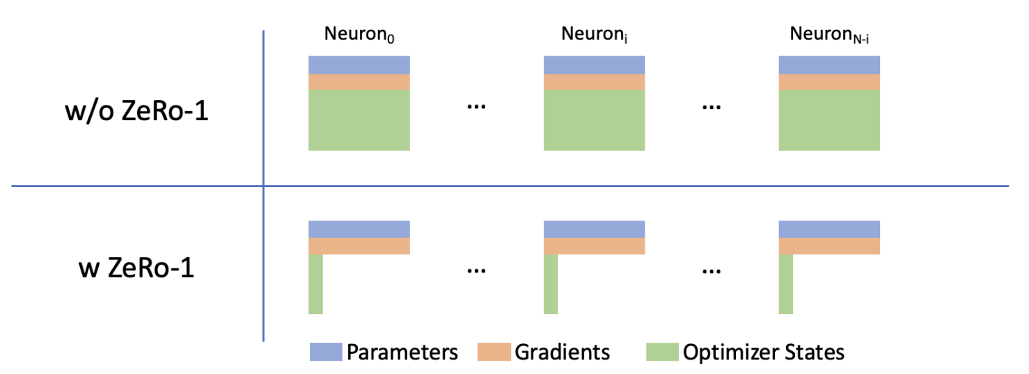
In total, the static memory required for training is:
\[M_{static} = (6 + \frac{10}{d})\frac{1}{t}P\]2.2 Activations Memory Estimation
Another one that takes up much memory is activations memory, which is the memory used for storing intermediate activation values during the forward and backward passes of the training process. I will use GPT-Next(LLaMA similar structure) as an example to explain how to estimate activations memory.
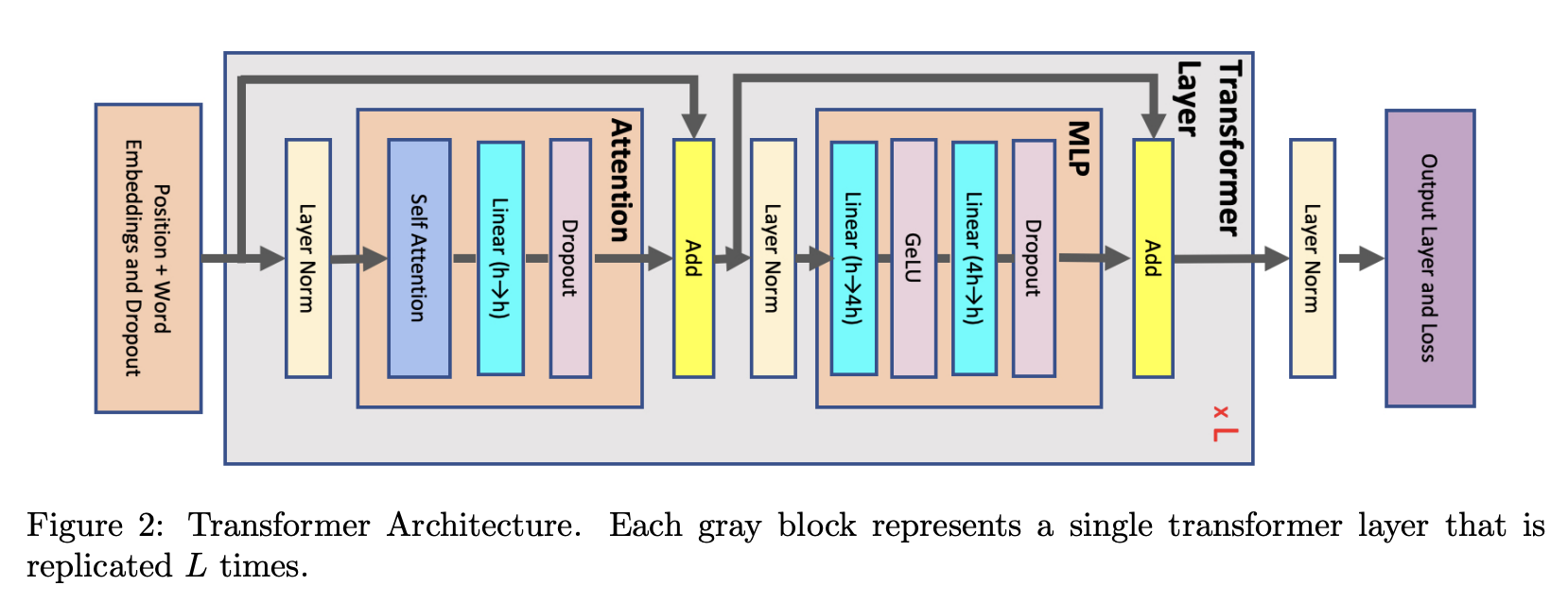
The figure above shows that each transformer layer consists of attention and an MLP block connected with two-layer norms. Below, we derive the memory required to store activations for each of these elements:
Attention block: includes self-attention followed by a linear projection and an attention dropout. The linear projection stores its input activations with size \(2sbh\), and the attention dropout requires a mask with size \(sbh\). The self-attention shown in the figure above consists of several elements:
- Query (Q), Key (K), and Value (V) matrix multiplies: We only need to store their shared input with size \(2sbh\).
- QKT matrix multiply: It requires the storage of both Q and K with a total size of \(4sbh\).
- Softmax: Softmax output with size \(2as^2b\) is required for back-propagation.
- Softmax dropout: Only a mask with size \(as^2b\) is needed.
- Attention over Values (V): We need to store the dropout output (\(2as^2b\)) and the Values(\(2sbh\)) and therefore need \(2as^2b + 2sbh\) of storage.
Summing the above values, in total, the attention block requires \(11sbh + 5as^2b\) bytes of storage.
MLP: The two linear layers store their inputs with size \(2sbh\) and \(2sbh_{ff}\). The SwiGLU non-linearity needs three \(2sbh_{ff}\) sized activations, one for the input and others for the dot product. Finally, dropout stores its mask with size \(sbh\). In total, the MLP block requires \(3sbh + 8sbh_{ff}\) bytes of storage.
Layer norm: Each layer norm stores its input with size \(2sbh\) and therefore in total, we will need \(4sbh\) of storage.
Summing the memory required for attention, MLP, and layer norms, the memory needed to store the activations for a single layer of a transformer network is:
Activations memory per layer = \(sbh(18 + 8\frac{h_{ff}}{h} + 5\frac{as}{h})\).
The majority of the required activation memory is captured by the equation above. However, this equation does not capture the activation memory needed for the input embeddings, the last layer norm, and the output layer cross-entropy. The input embeddings dropout requires \(sbh\) bytes of storage; the last layer-norm requires \(2sbh\) storage. Finally, the cross entropy loss requires storing the logits, which are calculated in a 32-bit floating point and, as a result, will require \(4sbv\) of storage. So the extra memory due to the input embeddings, the last layer-norm, and the output layer is \(3sbh + 4sbv\).
Adding the above two equations, the total memory required for activations is:
\[M_{activation} = sbhL(18 + 8\frac{h_{ff}}{h} + 5\frac{as}{h}) + 3sbh + 4sbv\]In addition, just like PaLM’s practice, Dropout can be omitted in pre-training, saving the activation memory brought by the dropout mask of input Embedding, Attention, and MLP. The corresponding formula is as follows:
\[M_{activation} = sbhL(16 + 8\frac{h_{ff}}{h} + 5\frac{as}{h}) + 2sbh + 4sbv\]One more thing, we still need to apply the NeMo optimization technique. NeMo uses selective activation recomputation (SAR) to reduce the memory required for storing activations by recomputing only a subset of the activations during the backward pass. And with tensor parallel SAR, the memory needed for storing activations is:
\[M_{activation} = sbhL(8 + (8 +8\frac{h_{ff}}{h})/t) + 2sbh + 4sbv/t\]This chapter contains many excerpts from Korthikanti et al., 2023; only in the MLP part there is a formula change because of the new activation function of GPT-Next.
2.3 Cross Entropy Overhead, PyTorch Overhead, and CUDA Context
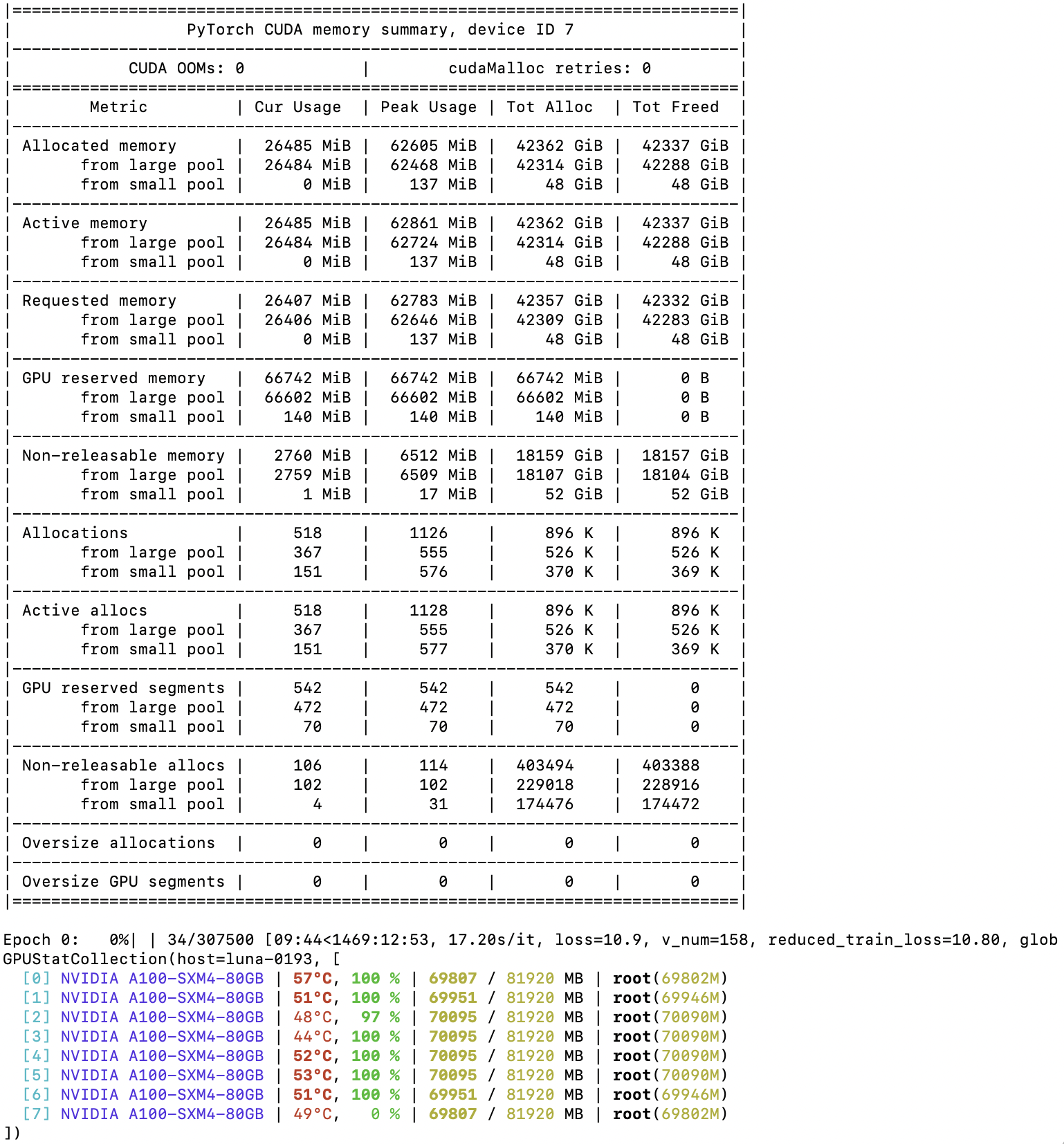
Except for static memory and activations memory, some memory is big enough to be considered.
The first one is cross entropy overhead, cross-entropy is calculated at the end of the forward pass, and its runtime memory will be accumulated on static memory and activations memory to form a memory peak. The memory required for cross-entropy has two parts, 32-bit floating point input with size \(4sbv/t\), and if we have tensor parallel, we need a communication buffer with size \(2sbv/t\) for parallel computing. So the memory required for cross-entropy is \(6sbv/t\).
The second one is PyTorch overhead, the memory obtained by the PyTorch memory allocator from CUDA but not used. We can calculate it by subtracting the memory occupied by tensors(peak value of PyTorch allocated memory) from the memory used by the PyTorch memory allocator(peak value of PyTorch reserved memory).
The last one is CUDA context, which the CUDA libraries like cuDNN, CUTLASS, and others usually use. We can calculate it by subtracting the memory used by the PyTorch memory allocator(peak value of PyTorch reserved memory) from memory used by nvidia-smi.
3 Experimental Validation of Memory Estimation
To validate the memory estimation derived in the previous sections, I will train some GPT models using the NeMo framework under different configurations. I will then observe the actual running memory of the training process and compare it with the memory estimation.
3.1 Experimental Setup
I selected three models for experimental configuration: gpt-1b, gpt-5b, and gpt-7b. They are all GPT-Next architectures(with rotary position embedding and LLaMA-like MLP block), and the experiment was completed on a DGX-A100.
The following table shows the hyperparameters of the three models:
| model | L | h | \(h_{ff}\) | v | parameters |
|---|---|---|---|---|---|
| gpt-1b | 24 | 2048 | 5440 | 50257 | 1.41E+09 |
| gpt-5b | 24 | 4096 | 10880 | 50257 | 5.23E+09 |
| gpt-7b | 32 | 4096 | 10880 | 50257 | 6.84E+09 |
Each model organizes multiple sets of tests. The test starts from the sequence length of 2048 and gradually increases. To test as close as possible to the actual use, I adjust the tp(tensor parallel world size) and micro-batch size according to the situation so that the training is always performed efficiently.
The following table shows the test configuration of the three models:
| parameters | sequence length | dp | tp | micro-batch size | Estimated Static Memory | Estimated Activation Memory | Estimated Cross-Entropy Overhead | Estimated Memory | ||
|---|---|---|---|---|---|---|---|---|---|---|
| gpt-1b | 2048 | 8 | 1 | 2 | 9.52 | 7.77 | 0.77 | 18.05 | ||
| gpt-1b | 4096 | 8 | 1 | 2 | 9.52 | 15.53 | 1.53 | 26.59 | ||
| gpt-1b | 8192 | 8 | 1 | 2 | 9.52 | 31.07 | 3.07 | 43.66 | ||
| gpt-1b | 16384 | 8 | 1 | 1 | 9.52 | 31.07 | 3.07 | 43.66 | ||
| gpt-1b | 32768 | 4 | 2 | 1 | 5.58 | 37.13 | 4.60 | 47.31 | ||
| gpt-1b | 65536 | 2 | 4 | 1 | 3.61 | 49.25 | 4.60 | 57.47 | ||
| gpt-5b | 2048 | 8 | 1 | 2 | 35.31 | 14.77 | 0.77 | 50.85 | ||
| gpt-5b | 4096 | 8 | 1 | 1 | 35.31 | 14.77 | 0.77 | 50.85 | ||
| gpt-5b | 8192 | 4 | 2 | 2 | 20.70 | 35.60 | 2.30 | 58.60 | ||
| gpt-5b | 16384 | 4 | 2 | 1 | 20.70 | 35.60 | 2.30 | 58.60 | ||
| gpt-5b | 32768 | 2 | 4 | 1 | 13.39 | 47.72 | 2.30 | 63.42 | ||
| gpt-5b | 65536 | 1 | 8 | 1 | 9.74 | 71.97 | 2.30 | 84.01 | ||
| gpt-7b | 2048 | 8 | 1 | 2 | 46.25 | 19.42 | 0.77 | 66.44 | ||
| gpt-7b | 4096 | 8 | 1 | 1 | 46.25 | 19.42 | 0.77 | 66.44 | ||
| gpt-7b | 8192 | 4 | 2 | 1 | 27.11 | 23.45 | 1.15 | 51.72 | ||
| gpt-7b | 16384 | 2 | 4 | 1 | 17.54 | 31.52 | 1.15 | 50.21 | ||
| gpt-7b | 32768 | 1 | 8 | 1 | 12.76 | 47.64 | 1.15 | 61.55 | ||
| gpt-7b | 65536 | 1 | 8 | 1 | 12.76 | 95.28 | 2.30 | 110.34 |
3.2 Results and Analysis
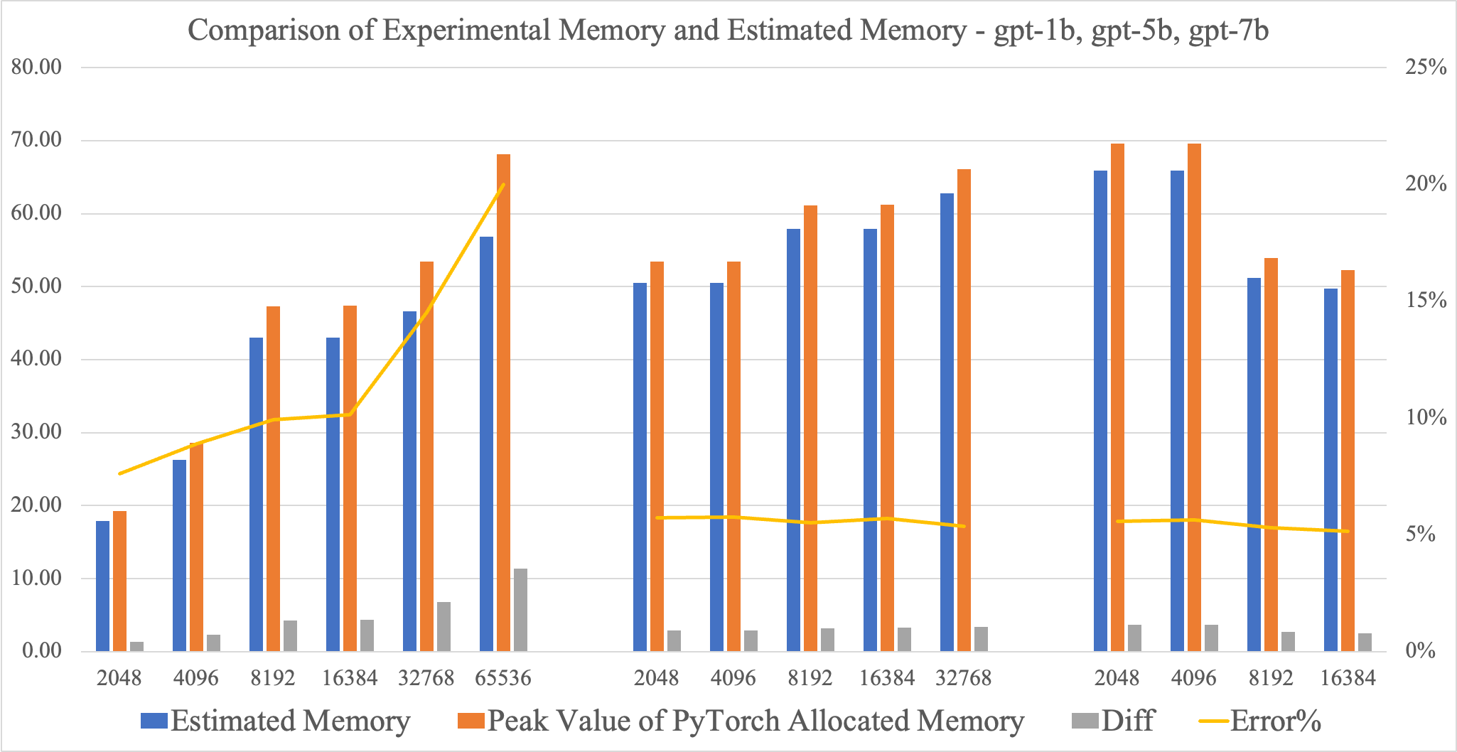
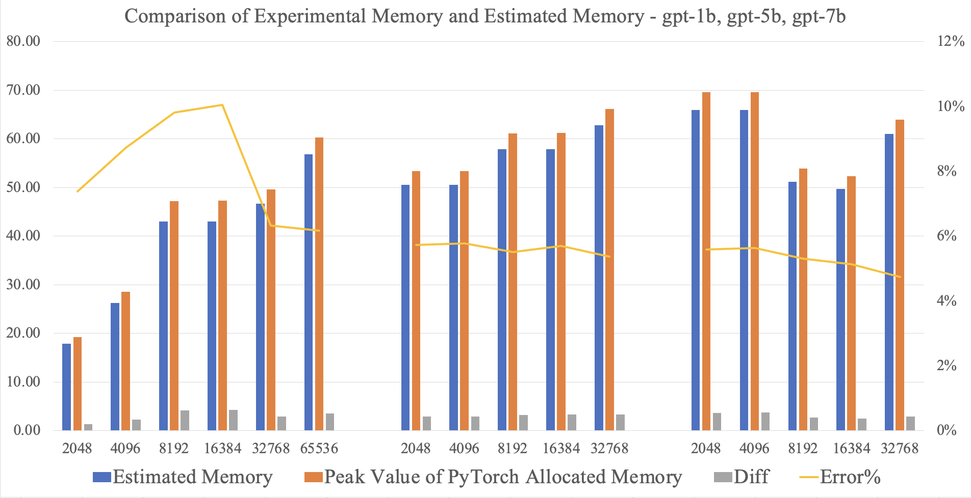
After experiments, I got the experimental results on the chart. The chart is divided into three parts. From left to right are the results of gpt-1b, gpt-5b, and gpt-7b. The deletion of gpt-1b 32k sequence length and gpt-5b 32k and 64k sequence length is due to OOM. The gray column is the difference between experimental memory and estimated memory, and the percentage represented by the yellow line is the ratio of the difference to estimated memory.
The estimation model performs well on gpt-5b and gpt-7b, with an error of about 5%. But in gpt-1b, there are more than 15% errors on 32k and 64k sequence length, and for gpt-7b 32k sequence length, the estimated memory is 61.55GB, lower than the 80GB GPU memory. It should not be OOM. To find the reason for this phenomenon, I used PyTorch’s memory snapshot tool to profile the gpt-1b 64k sequence length training and found unexpected metrics.
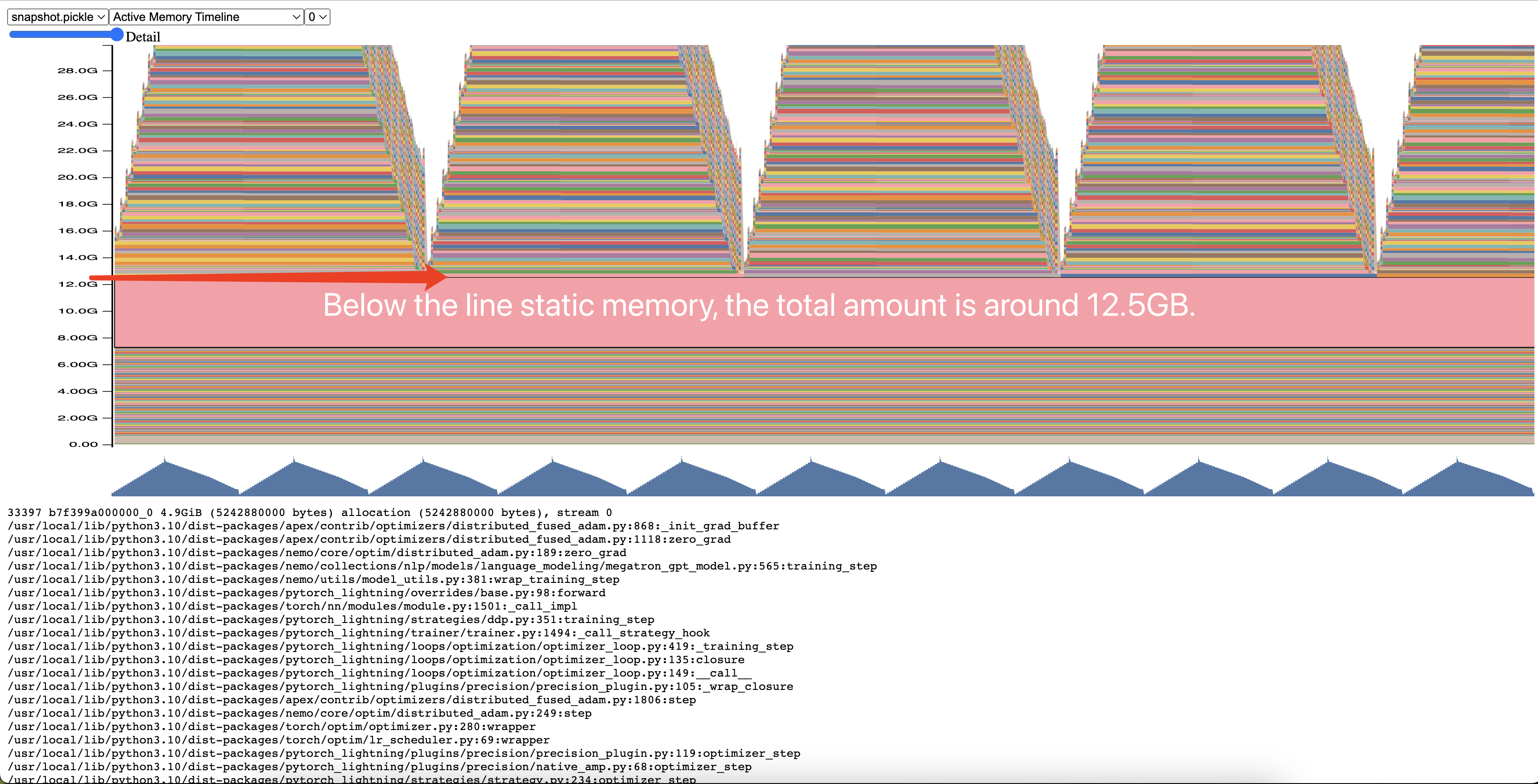
The memory snapshot tool can see the change in PyTorch memory over time. In the figure, the part that does not change in the forward and backward process is the static memory. Our estimated static memory is 3.61GB, but the actual static memory is 12.5GB, which is far exceeded our expectations.
After some analysis, I found that this phenomenon is due to the special bucket mechanism of the optimizer apex.distributed_fused_adam. The apex.distributed_fused_adam bucket mechanism is designed for parameter updates. When updating parameters, doing gradient updates one by one will launch many small kernels, which is inefficient, in place apex.distributed_fused_adam gradients are placed in continuous buffers(bucket), and many small kernels can be combined into one big kernel to improve efficiency. But there is also a problem with this design. The bucket has a fixed length, and if there are few parameters and the bucket is large, it will cause waste. Unfortunately, I used a 200MB bucket in gpt-1b, and tensor parallel will make the parameters on each rank tiny. When tp=4, a 50MB bucket is enough, which is the cause I used four times the estimated memory.
We can calculate the appropriate bucket size by the formula \(4 * P / Lt\), where \(P\) is the number of parameters, \(L\) is the number of transformer layers, and \(t\) is the tensor parallel size. It needs to be divided by \(L\) because NeMo will make a bucket for each layer of the transformer, and \(P/t\) is the total number of parameters on each instance when using tensor parallel, and \(4\) is for 32-bit floating point datatype.
After correcting the optimizer bucket size, I re-did the experiment, and the result was as expected.
4 PyTorch Profiling Tools
In the above experimental process, PyTorch’s profiling tool gave me much help. In this section, I will introduce the PyTorch profiling tools in detail.
There are two handy PyTorch profiling tools that I recommend to you, one is PyTorch profiler, and the other is PyTorch memory snapshot.
4.1 PyTorch Profiler
PyTorch profiler is a tool that can help us analyze the time cost of each operation in the training process. It can be used in two ways, one is to use the torch.profiler.profile API to profile the code, and the other is to use the torch.profiler.Profiler API to profile the code. The former is more convenient, but the latter is more flexible.
The following is an example of using the torch.profiler.profile API to profile the code:
with torch.profiler.profile(
    activities=[
        torch.profiler.ProfilerActivity.CPU,
        torch.profiler.ProfilerActivity.CUDA,
    ],
    schedule=torch.profiler.schedule(
        wait=2,
        warmup=2,
        active=2,
        repeat=1,
    ),
    on_trace_ready=torch.profiler.tensorboard_trace_handler('./log'),
    record_shapes=True,
    profile_memory=True,
    with_stack=True,
) as profiler:
    model.train()
    for batch_idx, (data, target) in enumerate(train_loader):
        if batch_idx == 10:
            break
        data, target = data.to(device), target.to(device)
        optimizer.zero_grad()
        output = model(data)
        loss = F.nll_loss(output, target)
        loss.backward()
        optimizer.step()
        profiler.step()
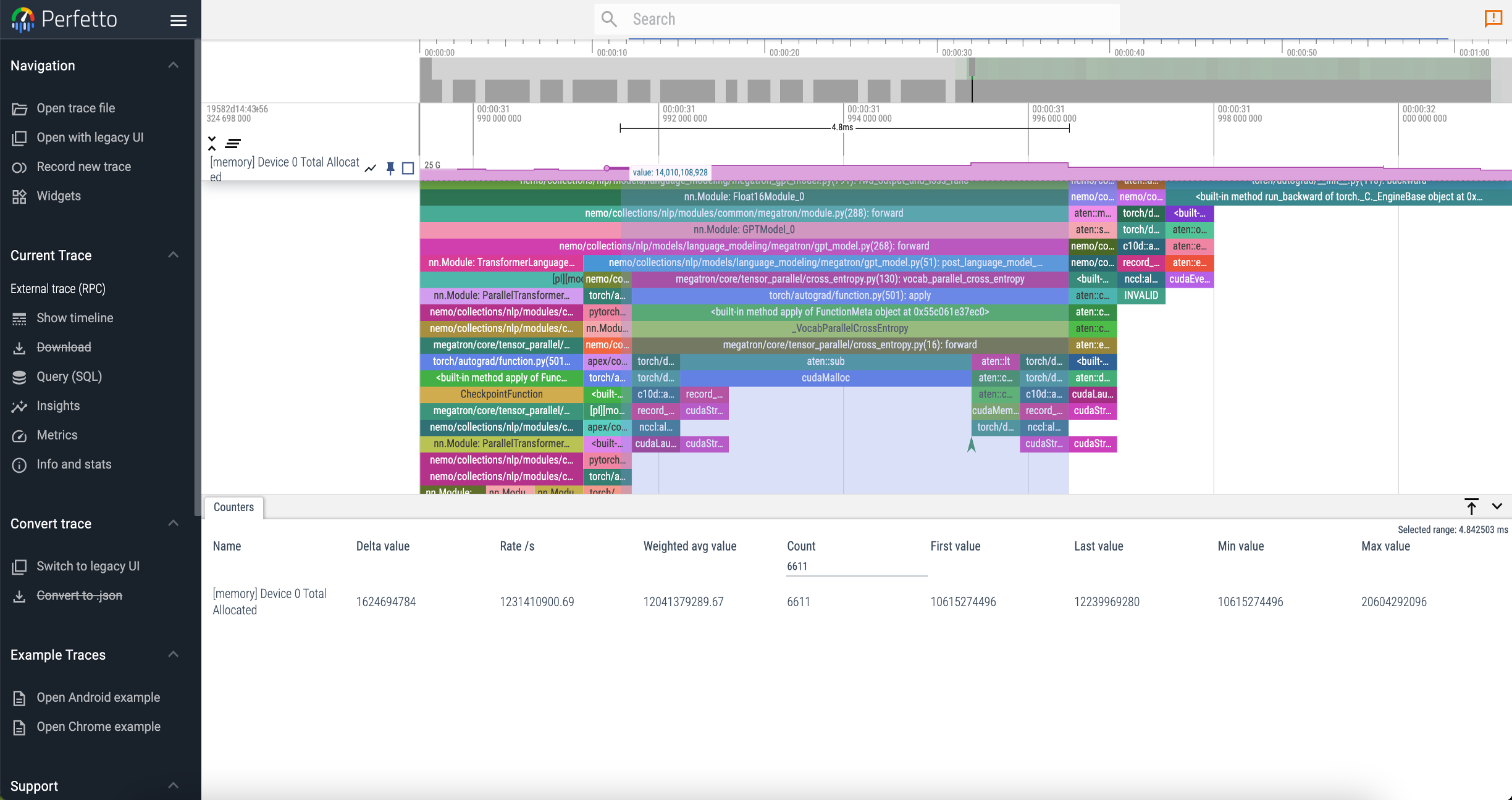
You can show trace event data(dump in “./log”) in chrome tracing GUI, for example, Perfetto UI, and then you can find helpful information like GPU kernel execution time, call stack, memory usage, etc.
4.2 PyTorch Memory Snapshot
When you do memory analysis, you can use PyTorch memory snapshot to help you. The PyTorch Memory Snapshot can give detailed trace events on the PyTorch memory allocator. It clearly shows you which memory blocks constitute the allocated memory at a particular moment and these memory blocks are allocated in which function.
To use PyTorch memory snapshot, you need to enable memory recording:
torch.cuda.memory._record_memory_history(True,
        # keep 100,000 alloc/free events from before the snapshot
        trace_alloc_max_entries=100000,

        # record stack information for the trace events
        trace_alloc_record_context=True)
You can get a memory snapshot by:
snapshot = torch.cuda.memory._snapshot()
Saving snapshot for latter analysis:
from pickle import dump
with open('snapshot.pickle', 'wb') as f:
    dump(snapshot, f)
With PyTorch’s visualization tool, you can visit it interactively in the browser.
$ wget https://raw.githubusercontent.com/pytorch/pytorch/master/torch/cuda/_memory_viz.py
$ python _memory_viz.py trace_plot snapshot.pickle -o trace.html
Interactive visualization of gpt-1b 64k sequence length’s memory snapshot here.
5 Limitations
The model object of the memory modeling is a LLaMA-like model, and it is assumed that the model adopts a standard hyperparameter configuration, and the number of model parameters is also large. For extreme configuration models or smaller-scale models, There will be prediction errors. In addition, the experiment was carried out on NeMo, and it cannot be guaranteed correct when using the same technology but different frameworks. In distributed technology, pipeline parallelism is not considered.
6 Discussion and Conclusion
I have been doing deep learning training for more than 3 years. Even though I have dealt with many cases, before doing this, I am not sure that I can predict the memory cost in training. The tools I used before have too much uncertainty. I have seen a lot of losses caused by cache and alignment, so I don’t believe that I can build a relatively accurate model.
I would like to praise Megatron and NeMo. They can model the memory more accurately as described in the Korthikanti paper. Although I experienced some twists and turns, I finally completed memory modeling for the LLaMA-like model in mixed precision, ZeRO, tensor parallel and data parallel.
However, NeMo’s distributed optimizer needs to be improved. The bucket mechanism has potential memory waste, and the value is not small. We can do some self-checks. We can report this information to the user if a lot of GPU memory is wasted.
Finally, regarding PyTorch, I would like to add that the memory counted by PyTorch’s new tool memory snapshot is extraordinary. Its measurement is different from the previous indicators. Its peak value is neither torch.cuda.max_memory_allocated() nor torch.cuda.max_memory_reserved(), although it is different from these two values are close but different. What is included in the memory counts is still a mystery, and there may be a chance to explore it later.
References
- Korthikanti, V.A., Casper, J., Lym, S., McAfee, L., Andersch, M., Shoeybi, M. and Catanzaro, B., 2023. Reducing activation recomputation in large transformer models. Proceedings of Machine Learning and Systems, 5.
- Visualizing PyTorch memory usage over time - Zach’s Blog
- Chowdhery, A., Narang, S., Devlin, J., Bosma, M., Mishra, G., Roberts, A., Barham, P., Chung, H.W., Sutton, C., Gehrmann, S. and Schuh, P., 2022. Palm: Scaling language modeling with pathways. arXiv preprint arXiv:2204.02311.